7.3 Confidence Intervals for Means

In chapter 4 we have seen how to compute the mean, median, standard deviation, and other descriptive statistics for a given data set, usually a sample from an underlying population. In this section we want to focus on estimating the mean of a population, given that we can compute the mean of a particular sample. In other words, if a sample of size, say, 100 is selected at random from some population, it is easy to compute the mean of that sample. It is equally easy to then use that sample mean as an estimate for the unknown population mean. But just because it's easy to do does not necessarily mean it's the right thing to do ...

For example, suppose we randomly selected 100 people, measured their height, and computed the average height for our sample to be, say, 164.432 cm. If we now wanted to know the average height of everyone in our population (say everyone in the US), it seems reasonably to say that the average height of everyone is 164.432 cm. However, if we think about it, it is of course highly unlikely that the average for the entire population comes out exactly the same as the average for our sample of just 100 people. It is much more likely that our sample mean of 164.432 cm is only approximately equal to the (unknown) population mean. It is the purpose of this chapter to clarify, using probabilities, what exactly we mean by "approximately equal".  In other words:

Can we use a sample mean to estimate an (unknown) population mean, and - most importantly - how accurate is our estimated answer.

Example: Consider some data for approximately 400 cars. We assume that this data has been collected at random. We would like to make predictions about all automobiles, based on that random sample. In particular, the data set lists miles per gallon, engine size, and weight of 400 cars, but we would like to know the average miles per gallon, engine size, and weight of all cars, based on this sample.

It is of course simple to compute the mean of the various variables of the sample, using Excel. For our sample data we find that:

mean gas mileage of the sample is 23.5 mpg with a standard deviation of 7.82 mpg, using 398 data values

But we need to know how well this sample mean predicts the actual and unknown population mean for the entire distribution. Our best guess is clearly that the average mpg for all cars is 23.5 mpg - it's after all pretty much the only number we have - but how good is that estimation?

<>In fact, we know more than just the sample mean. We also know that all sample means are distributed normally, according to the Central Limit Theorem, and that the distribution of all sample means (of which ours is just one) is normal with a mean of 23.5 mpg and a standard deviation of 7.82 / sqrt(398).

Using that information, let's make a quick d-tour into "mathematics land" - we will in a minute list a recipe for what we need to do, but for now, bear with me:

• Let's say we want to estimate an (unknown) population mean so that we are, say, 95% certain that the estimate is correct (or 90%, or 99%, or any other pre-determined notion of certainly we might have).
• To provide a reasonable estimate, we need to compute a lower number a and an upper number b in such a way as to be 95% sure that our (unknown) population mean is between a and b.

That interval (a, b) is known as a 95% confidence interval for the unknown mean.

• Using standard probability notation we can rephrase this: we want to find a and b so that P(a < m < b) = 0.95, i.e. the probability that the (unknown) mean is between a and b should be 0.95, or 95%, which could be depicted as follows:

  

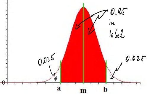
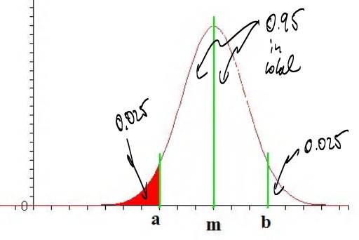
• Using symmetry and focusing on the part of my distribution that we can compute with Excel, this is equivalent to finding a value of a such that P(x < a) = 0.025, where x is normally distributed, as in the following picture:
  

  

If the distribution had mean 0 and standard deviation 1 we could use some trial-and-error in Excel to compute the desired number a - note that if we assume that the mean was 0, a should be negative. In other words, we use Excel to compute NORMDIST(a, 0, 1, TRUE), where we guess some values of a:

• NORMDIST(-0.5,0,1,TRUE) = 0.308537539 (too much probability)
• NORMDIST(-1.5,0,1,TRUE) = 0.066807201 (still too much)
• NORMDIST(-2.0,0,1,TRUE) = 0.022750132 (now it's too little)
• NORMDIST(-1.9,0,1,TRUE) = 0.02871656 (again, too much)
• NORMDIST(-1.95,0,1,TRUE) = 0.02558806 (a little too much)
• NORMDIST(-1.96,0,1,TRUE) = 0.024997895 (just about right)

Thus, if the mean was 0 and the standard deviation was 1, the number a = -1.96 would be just about right, and using symmetry we can conclude that b = +1.96. However, we don't know the mean and standard deviation of our population, so what can we do ... Central Limit Theorem to the rescue!

According to the Central Limit Theorem, the mean and standard deviation of the distribution of all sample means is m and s / sqrt(N), where m is the sample mean and s is the sample standard deviation. Thus, the mean we are supposed to use is the sample mean m and the standard deviation s / sqrt(N), according to the Central Limit Theorem. Putting everything together, we found that we have computed a 95% confidence interval as follows:

from m - 1.96 * s / sqrt(N) to m + 1.96 * s / sqrt(N)

Note: The term s / sqrt(N) is also known as the Standard Error

The above explanation is perhaps somewhat confusing, and there are some parts where I've glossed over some important details. But the resulting formulas are simple, and those formulas will be what we want to focus on. In addition to the number 1.96 that we have derived for a 95% confidence interval, other numbers can be derived in a similar way for the 90% and 99% confidence intervals:

Confidence Interval for Mean (large sample size N > 30)

Suppose you have a sample with N data points, which has a sample mean m and standard deviation s. Then:

• To compute a 90% confidence interval for the unknown population mean, compute the numbers:

  m - 1.645 * s / sqrt(N) and m + 1.645 * s / sqrt(N)

  Then there is a 90% probability that the unknown population mean is between these values.
  
  
• To compute a 95% confidence interval for the unknown population mean, compute the numbers:

  m - 1.96 * s / sqrt(N) and m + 1.96* s / sqrt(N)

  Then there is a 95% probability that the unknown population mean is between these values.
  
  
• To compute a 99% confidence interval for the unknown population mean, compute the numbers:

  m - 2.58 * s / sqrt(N) and m + 2.54 * s / sqrt(N)

  Then there is a 99% probability that the unknown population mean is between these values.

Using these formulas we can now estimate an unknown population mean with 90%, 95%, or 99% certainty. Other percentages are also possible, but these are the most frequently used ones.

Returning to our earlier example, where m = 23.5, s = 7.82, and N = 398 we have:

• 90% confidence interval: from 23.5 - 1.645 * 7.82 / sqrt(398) =  22.85 to 23.5 + 1.645 * 7.82 / sqrt(398) = 24.14, thus:
  we are 90% certain that the average mpg for all cars is between 22.85 and 24.14
• 95% confidence interval: from 23.5 - 1.96 * 7.82 / sqrt(398) = 22.73 to 23.5 + 1.96 * 7.82 / sqrt(398) = 24.27, thus:
  we are 95% certain that the average mpg for all cars is between 22.73 and 24.27
• 99% confidence interval: from 23.5 - 2.54 * 7.82 / sqrt(398) = 22.5 to 23.5 + 2.54 * 7.82 / sqrt(398) = 24.4, thus:
  we are 99% certain that the average mpg for all cars is between 22.5 and 24.4

Note that a 99% confidence interval is large - i.e. includes more numbers - than a 90% confidence interval. That makes sense, since if we want to be more certain, we must allow for more values. Ultimately, a 100% confidence interval would simply consist of all possible numbers, or in an interval from -infinity to +infinity . That would certainly be correct, but is not very useful for practical applications.

While the above calculations can easily be done with a calculator (or Excel), our favorite computer program Excel provides - yes, you might have guessed it - a quick shortcut to obtain confidence intervals. We will proceed as follows:

• Load the above data into Excel
• Select "Data Analysis..." from the "Tools" menu entry and select "Descriptive Statistics"
• Select as input range the first few columns, including "Miles per Gallon", "Engine Size", "Horse Powers", and "Weight in Pounds".

  Note that we actually are not interested in "Horse Powers" but the input data range must consist of consecutive cells so we might as well include "Horse Powers" but ignore it in the final output. We should check the "Labels in First Row" box as well as "Summary Statistics" and "Confidence Level for Mean: " in the "Output options" section. We need to enter a level of confidence for the "Confidence Level for Mean". Common numbers are 90%, 95%, or 99% - we will explain the differences below again, or see the discussion above.

  

  For now, make sure that the figures are as indicated above.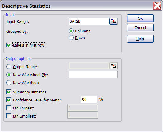
• Click on "OK" to see the following descriptive statistics (similar to what we have seen before):

What this means is that the sample mean of, say, "Mile per Gallon" is 23.5145. That sample mean may or may not be the same as the average MPG of all automobiles. But we have also computed a 90% confidence interval, which means, in this case, the following:

Under certain assumptions on the distribution of the population, we predict - based on our sample of 393 cars - that the average miles per gallon of all cars is somewhere between 23.5145 - 0.6459 = 22.87 and 23.5145 + 0.6459 = 24.16, and we are 90% certain that this answer is correct.

Please note that this 90% confidence interval is slightly different from the confidence interval we computed previously "by hand". That is no coincidence, because the derivation of the formulas for confidence intervals uses the Central Limit Theorem and that theorem, in effect, states that the distribution of the sample means is approximately normal. However, that approximation works best the larger N (the sample size) is. Excel uses a slightly different method to compute confidence intervals:

• If N is sufficiently large (30 or more) the "manual" method and Excel's method agree closely. In this case the method is based on the standard normal distribution
• If N is small (less than 30) the "manual" method is no longer appropriate and you should use Excel's method instead. In this case the method is based on the Student's T Distribution
  

Example: According to Excel, the average engine size in our sample of size N = 398 is 192.67 cubic inches, with a standard deviation of 104.55 cubic inches. Use these statistics to manually compute a 90% confidence interval. Then compare it with the figure Excel produces for the same interval.

• To compute a 90% confidence interval manually:
  
• from m - 1.645 * s / sqrt(N) to m + 1.645 * s / sqrt(N)
• from 192.67 - 1.645 * 104.55 / sqrt(398) to 192.67 + 1.645 * 104.55 / sqrt(398)
• from 192.67 - 8.62 to 192.67 + 8.62
• from 184.05 to 201.29
• To compute a 90% confidence interval using Excel
• as the above output shows, the mean m = 192.67 while the confidence level (90%) is 8.64
• from 192.67 - 8.64 to 192.67 + 8.64
• from 184.03 to 201.31
  

<>Thus, since the sample size is large (certainly larger than 30) the intervals computed manually and with Excel are virtually identical. For the picky reader, note that Excel's interval is slighly larger, so it's slightly more conservative than the manual computation, but the difference in this case is neglibile.

Similarly, according to Excel the average weight in pounds of all cars is 2969.5161 - 69.5328 and 2969.5161 + 69.5328, and we are 90% certain that we are correct.

To recap: Instead of providing a point estimate for an unknown population mean (which would almost certainly be incorrect) we provide an interval instead, called confidence interval. Three particular confidence intervals are most common: a 90%, a 95%, or a 99% confidence interval. That means that:

• if the interval was computed according to a 90% confidence level, then the true population mean is between the two computed numbers with 90% certainty, and the probability that the true population mean is not inside that interval is less than 10%
• if the interval was computed according to a 95% confidence level, then the true population mean is between the two computed numbers with 95% certainty, and the probability that the true population mean is not inside that interval is less than 5%
• if the interval was computed according to a 99% confidence level, then the true population mean is between the two computed numbers with 99% certainty, and the probability that the true population mean is not inside that interval is less than 1%

Example: Suppose we compute, for the same sample data, both a 90% and a 99% confidence interval. Which one is larger ?

To answer this question, let's compute both a 90% and a 99% confidence interval for the "Horse Power" in the above data set about cars, using Excel. The procedure of computing the numbers is similar to the above; here are the answers:

• the sample mean for the "Horse Power" is 104.8325
• the 90% confidence level results in 3.1755, so that the 90% confidence interval goes from 104.8325 - 3.1755 to 104.8325 + 3.1755, or from 101.657 to 108.008
• the 99% confidence level results in 4.9851, so that the 99% confidence interval goes from 104.8325 - 4.9851 to 104.8325 + 4.9851, or from 99.84735 to 109.8176

That means, in general, that a 99% confidence interval is larger than a 90% confidence interval. That actually makes sense: if we want to be more sure that we have captured the true (unknown) population mean correctly, we need to make our interval larger. Hence, a 99% confidence interval must include more numbers than a 90% confidence interval; it is therefore wider than a 90% interval.