7.2 The Central Limit Theorem

In the previous section we first saw that we can use frequency distributions to compute probabilities of various events. Then we saw that we could use various normal distributions as a shortcut to compute those probabilities, which was very convenient. Using that technique we were able to compute all kinds of probabilities just based on the fact that we computed a sample mean and sample standard deviation, and then assumed, more or less, that the (unknown) distribution of the variable in question was normal, more or less, with the computed mean and standard deviation as the right parameters.

But this works if we assume the original distribution is (approximately) normal, so what we are hoping for is some mathematical justification that says, in effect, that most distributions - in some sense - are "normal". Such a theorem does indeed exist, and it is one of the corner-stones of statistics: the Central Limit Theorem. It has many practical and theoretical implications, such as it will provide us with a theoretical justification of using a normal distribution to compute certain probabilities.

In this course we will simply state the theorem without any proof. In more advanced courses we would provide a justification and/or mathematical proof of the theorem, but for our current purposes it will be enough to understand the theorem and to apply it in subsequent chapters. If we want to talk colloquially, we have actually already seen the Central Limit Theorem - in the previous chapter we noted: most histograms are (more or less) bell-shaped, which is in fact one way to state the Central Limit Theorem:

Central Limit Theorem, colloquial version 1

Most histograms (frequency distributions) are normal

To state this theorem precisely, we need to specify, among other things, exactly which normal distribution we are talking about, and under what circumstances we are considering samples.

Central Limit Theorem for Means

Suppose x is a variable for a population whose distribution has a mean m and standard deviation s, but whose shape is unknown. Suppose further we repeatedly select random samples of size N from that population and compute the sample mean each time we do this. Finally, we plot the distribution (histogram) of all these sample means.

Then the conclusion is that the distribution of all sample means is a normal distribution (bell shaped) with mean m (the original mean) and standard deviation s / sqrt(N)

This theorem is perhaps somewhat hard to understand, so here is a more colloquial restatement of the theorm.

Central Limit Theorem, colloquial version 2

No matter what shape a distribution for a population has, the distribution of means computed for samples of size N is bell shaped (normal). Moreover, if we know the mean and standard deviation of the original distribution, the mean for the sample means will be the same as the original one, while the new standard deviation will be the original one divided by the square root of N (the sample size).

The importance of this theorem is that it allows us to start with an arbitrary distribution, yet use the normal distribution with appropriate mean and standard deviation, to perform various computations. Since Excel contains the NORMDIST function, we can therefore compute probabilities for many distributions, regardless of whether they are normally distributed or not.

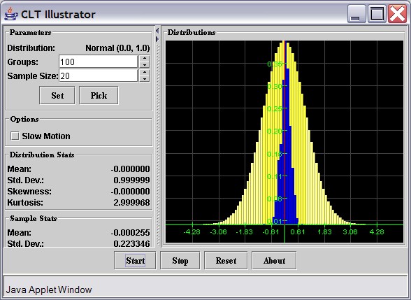
If you want to see the Central Limit Theorem in action, check out the Central Limit Applet (it requires that you have the Java Plug-in version 1.4 or better installed, which you could download here). Try the following:

• Click on the above link for the Central Limit Theorem applet
• You should see two buttons - click on the "Start CLT Applet" button (the page(s) might take a few minutes to initialize)
  

When you click "Start", the program will pick a random sample from a population, compute the mean, and mark where that mean is on the x-axis to start a frequency distribution for the sample mean. Then the program picks another random sample, computes its mean, marks it in blue, and continues in that fashion (you could check off the "Slow Motion" checkbox to see what the program does in slow motion"). After the program is running for a while, notice that the blue bars are slowing building up to a real frequency distribution (the yellow bars underneath show the distribution of the underlying population from which the random samples are selected. Now try the following:

• Let the program run (at regular speed) for a while. What shape is the distribution of the random samples (blue bars), at least approximately?
• Experiment with different distributions (click on [Pick] to choose another distribution). What shape does the distribution of the sample means (blue chart) have when you pick other distributions for the population? Is that true regardless of the underlying population distribution (yellow chart)?
• What is the mean for the distribution of the sample means (blue chart) in relation to the mean of the distribution of the original distribution (yellow chart)? The figures for the sample means are shown in the category "Sample Stats", but make sure to run the program for a while before looking at the numbers. Note that these numbers represent the "sample mean" for the distribution of all sample means, and the "sample standard deviation" for the distribution of all sample means (yes, it sounds odd, but that's what it is).
  
• Is there a relation between the standard deviation of the sample means (blue chart) and that of the original population (yellow chart)? Experiment with sample sizes 16, 25, 36, 49, and 64 to find the relation, but make sure to press the Reset button before using new parameters or sample sizes, and let the program run for a while before estimating the sample stats.

If you have done everything correctly, you have just discovered the Central Limit Theorem! On the other hand, .if you have any trouble with that applet, or if you are not exactly sure what it shows and how it works, don't worry. In this class we are interested in the consequences of the Central Limit theorem, which we will discuss next, and not in that theorem in and of itself.

For the record, there is an additional Central Limit Theorem for taking sums of samples, but we will not need that in our discussions.