5.4 Chi-Square Test for Crosstab Data
In the previous section we computed crosstab tables, relating two categorical variables with each other. A natural question to ask now is:
Is there a relationship between two (categorical) variables, or do they appear to be independent?
The complete answer to this question would take us into the realm of hypothesis testing, which we have not yet introduced. For example, what exactly do we mean by "independent". But the question is intuitively easy to understand, so we will give a brief discussion on how to answer the above question without covering all of the mathematical details.
Example: Consider the crosstabs table we generated before, relating income with sex for a particular company, using the data file Selected Employees. The table we generated (using raw numbers, not row or column percentages) looked as follows:
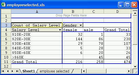
A natural and interesting question is: "Is there a relationship between salary and sex (the row and column variables) or do the two variables appear to be independent of each other".
To answer this question we assume that the row and column variables are independent, or unrelated. If that assumption was true we would expect that the values in the cells of the table are balanced.
Actual versus Expected - the Theory
To determine what we mean by balanced, let's take a simple example with two variables, sex and smoking, for example. We are interested in figuring out whether there is a relation between sex (male/female) and smoking (yes/no), or whether the two variables are independent of each other. We therefore conduct an experiment and ask a randomly selected group of people for their sex and whether they smoke. Then we construct the corresponding crosstabs table. Let's say we get a tables as follows (the actual numbers are fictitious):
Male Female Totals Smoking 30 5 35 Not smoking 10 55 65 Totals 40 60 100
Of the 35 people that are smoking, 30 of them are male. Conversely, of the 65 people that are not smoking, 55 of them are female. Such an outcome - using common sense - would suggest that there is a relation between smoking and sex, because the vast majority of smokers is male, while the majority of non-smokers is female.
On the other hand, we might have gotten a table like this (again with fictitious numbers):
Male Female Totals Smoking 22 18 40 Not smoking 26 34 60 Totals 48 52 100
Now the smokers and non-smokers are divided pretty much evenly among men and woman, suggesting perhaps that the two variables are independent of each other (a person's sex does not seem to have an impact on their smoking habit).
Now let's look exactly how a balanced table should look like if we assume that two variables are indeed independent. Suppose we are again conducting our experiment and select some random sample, but for now we only look at totals for each variable separately (the actual numbers are once again fictitious). Suppose, for example:
- number of smokers is 30, number of non-smokers is 70
- number of males is 40, number of females is 60
- total number of data values (subjects) is 100
With this information we could construct a crosstabs tables as follows:
Male Female Totals Smoking
30 Not smoking
70 Totals 40 60 100
But what kind of distribution in the various cells would we expect if the two variables were independent?
- We know that 30 of 100 (30%) are smoking; there are 40 males and 60 females - if male and female had nothing to do with smoking (the variables were independent) that we would expect that 30% of the 40 males are smoking, while 30% of the 60 females were smoking.
- We also know that 70 of 100 (70%) are not smoking; there are 40 males and 60 females - if the two variables were independent, I would similarly expect that 70% of the 40 males were not smoking and 70% of the 60 females were not smoking
Under the assumption of independence I would expect my table to look as follows:
Male Female
Totals
Smoking 30/100 * 40 = 12 30/100 * 60 = 18 30 Not smoking 70/100 * 40 = 28 70/100 * 60 = 42 70 Totals 40 60 100
In other words, if a crosstabs table with 2 rows and 2 columns has a row totals r1 and r2, respectively, and column totals c1 and c2, then if the two variables were indeed independent we would expect the complete table to look as follows:
X Y Totals A r1 * c1 / total r1 * c2 / total r1 B r2 * c1 / total r2 * c2 / total r2 Totals c1 c2 total
But now we have a procedure to test whether two variables are independent:
- Create a crosstabs table as usual, called the actual or observed values (not percentages)
- Create a second crosstabs table where you leave the row and column totals, but erase the number in the individual cells.
- If
the
two variables were independent, you would expect the entry in the i-th
row and j-th column to be
(total of row i) * (total of column j) / (overall total)
Fill in all cells in this way and call the resulting crosstabs table the expected values table - Now here is the clue: if the actual values are very different from the expected values, the conclusion is that the variables can not be independent after all (because if they were independent the actual values should look similar to the expected values).
Actual versus Expected - the Example
Now lets' return to the original examples of determining whether sex (gender) and salary level are independent of each other or not for the particular company studied. According to our theoretical discussion, we create a second table with the same number of rows and columns (and labels) and name that table "Expected Values", while the original table will be named "Actual Values". We simply copy-and-paste the original table and erase the "inside cell" so we can recompute them (do not copy the very top line of the original table).
Note that the table with actual values must contain counts, not percentages
In the table of expected values, each entry is computed as the product of the row and column total for that cell, divided by the overall total. The next picture illustrates these computations:
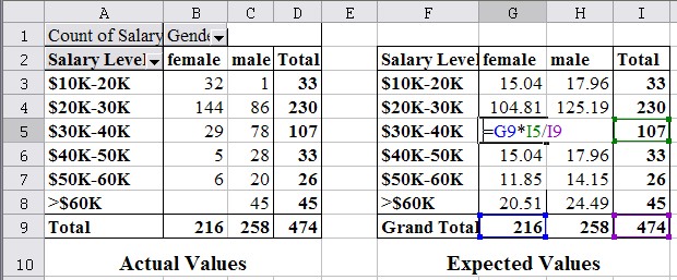
For example, the entry in cell G5 (column G, row 5) of the Expected Values table is the product of the column G total (cell G9) times the row 5 total (cell I5) divided by the overall total (cell I9). Similarly, the entries of the expected values are:
| Value of cell G3 = G9 * I3 / I9 | Value of cell H3 = H9 * I3 / I9 |
| Value of cell G4 = G9 * I4 / I9 | Value of cell H4 = H9 * I4 / I9 |
| Value of cell G5 = G9 * I5 / I9 | Value of cell H5 = H9 * I5 / I9 |
| ... | ... |
If we compare the values, we see that of the people making $60K or more, fewer than expected are female (0 versus 20.51) while more than expected are male (45 versus 24.49). On the other hand, in the low-income category of $10-$20K, more than expected are female (32 versus 15.04) while fewer than expected are male (1 versus 17.96). That seems to point towards a gender bias for salaries, i.e. women make less money than men as a rule, or to phrase it differently: the row and column variables do not seem independent of each other; rather, there seems to be a dependence between them. The next paragraphs will describe how to quantify such a conclusion of independence or dependence.
Now we have the actual values versus the expected values, where the expected values were computed under the assumption that the two variables are independent.
- If we compute the sum of all differences(*) between the actual and expected values, then it seems natural that if that sum was small, actual and expected values are close, which should be evidence for the variables to indeed be independent.
- If, however, the sum of differences(*) between actual and expected values is large, something is wrong. There is nothing we can do about the actual data values (they happen to be what we actually observed) something must be wrong with the expected values - but they were computed under the assumption of independence, which must therefore be wrong.
- if the sum of differences(*) between actual and expected values is "small", the assumption of independence is valid
- If the sum of differences(*) between actual and expected values is "large", the assumption of independence is invalid, hence there must be a relation between the variables
The big question left is: when is the difference small enough to accept the independence assumption, and when is the difference so large that we can no longer assume independence and must therefore accepted dependence. The answer to this question is provided by the Chi-Square test.
(*) We don't really need the sum of differences, because then negatives and positives would cancel each other out. Instead, we square all differences before adding them up to eliminate possible negative signs. Fortunately, though, Excel will handle the details of our computation.
The Chi-Square Test
The Chi-Square test computes the sum of the differences between actual and expected values (or to be precise the sum of the squares of the differences) and assign a probability value to that number depending on the size of the difference and the number of rows and columns of the crosstabs table.
- If the probability value p computed by the Chi-Square test is very small, differences between actual and expected values are judged to be significant (large) and therefore you conclude that the assumption of independence is invalid and there must be a relation between the variables. The error you commit by rejecting the independence assumption is given by this value of p.
-
If the probability value p computed by the Chi-Square test is large, differences between actual and expected values are not significant (small) and you do not reject the assumption of independence, i.e. it is likely that the variables are indeed independent.
To compute the value of p, use the Excel function =chitest(actual_range, expected_range)
Now we can finish the above example: we used the Selected Employees data to generate the crosstabs table:

First we copy this table of actual counts to a second table (IMPORTANT: DO NOT COPY THE TOP ROW OF THE TABLE) to another table and compute the expected values:

Please not that all expected values are bigger than 5 (the smallest expected value is 15.04), so the Chi-Square test is applicable. Thus, in an empty cell, enter the Chi-Square test function:
=chitest(B3:C8, G3:H8)
In the above case Excel computes that value to p = 1.91E-22, which is scientific notation for 0.00000000000000000000191. Thus, p is most definitely small and hence we conclude that there is a relation between the two variables sex and salary. In other words, the salary level in this particular company does depend on the sex of the employees. Since p is so close to zero our error is close to zero as well, so we are pretty certain that our conclusion is correct.
Example: Using the data from Selected Employees, is there a relation between salary and years of schooling?
We first use the data to create a crosstabs table of salary versus years of schooling, as in the previous section:
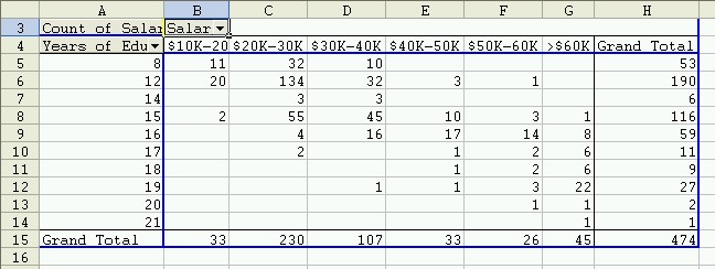
Next we copy this table (without copying the top row) and compute the expected values (a lot of work) as well as the Chi-Square test value p:
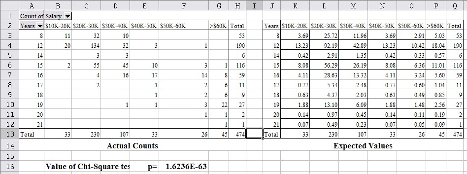
Again the value of p is for all intent and purposes zero (it's 0.00...0016236) so we could with high certainty conclude that there is a relation between years of education and salary level (in other words, you generally speaking make more money with a college degree than without, just like your parents told you).
BUT we failed to check if the expected values pass our "rule-of-thumb" test. In fact, many of the expected values are very small, and are certainly smaller than 5. Thus, in this case the Chi-Square test is not reliable and we should not believe its conclusions since the assumptions of the test were not satisfied! That does not mean our conclusion of dependence (or relationship) was invalid, it simply means we should not apply this test at all to draw any conclusions. To remedy the problem, you could re-categoroze the data by using fewer groups so that hopefully the expected values in the new tables will all be above 5 - but we made our point and won't pusue this any further. Instead, here is another example.
Example: Every year there are large-scale surveys, selecting a representative sample of people in the US and asking them a broad range of questions. One such survey is the General Social Science (GSS) survey from 1996 (which contains mostly categorical data). Use the data (which is real-life data from 1996) to analyze if there is a relation between party affiliation and people's opinion on capital punishmend
After downloading and opening the GSS96-selected.xls data file, we construct a crosstabs table for "Party Affil" and "Capital Punishment" as described in previous sections. Then we copy the table (of actual values) to a second table and construct the expected values as described above. Finally, we use the chitest Excel function to compute the value of p. Here are the resulting figures:
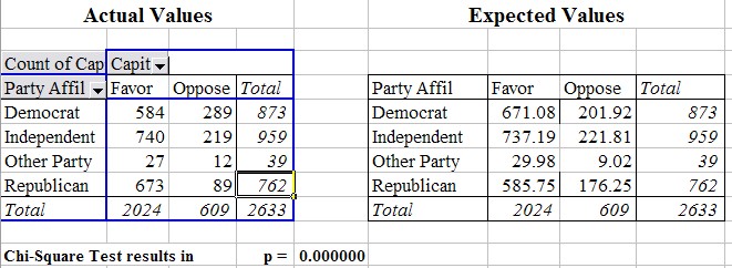
This time the smallest expected value is 9.02, which is above 5 so that it is valid to apply our Chi-Square test. Again p is very close to zero, stating that there is a relation between party affiliation and opinion on capital punishment. In fact, if you compare the actual versus expected values for the Democrats you can see that fewer democrats than expected favor the death penalty, while more than expected oppose it. For Republicans it is just the other way around. For independent and people with other party affiliations there seems to be little difference between actual and observed values.
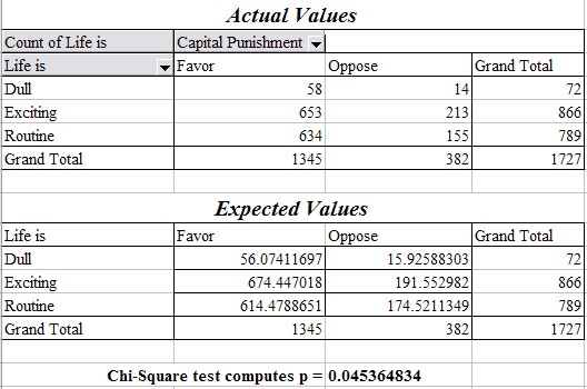
So far in all our examples the variables were dependent (probably). Of course that is not always the case. For example, if we setup the corresponding tables for actual and expected values for the data from the GSS96 survey relating "Life is" with opinion on "Capital Punishment", we see that the computed p value is p = 0.045, which means that if we did reject the assumption of independence and hence stated that the outlook on life and the opinion on capital punishment are related, we would make an error of 4.5% - that might be more than we are willing to accept (see figure below).
Finally, note that the Chi Square Test for crosstabs tables, as described here, checks whether two variables are independent of each other or not. If the test results in our conclusion that two variables are related, then the next question is: how strong are they related. There are different statistical procedures that allow you to decide about the strength of a relation ship, but for categorical data Excel does not provide the necessary functions or procedure to quickly perform these necessary computations.
To analyze the strength of a possible relation between two variables we will restrict ourselves to numerical variables and move on to the next chapter.